Introduction
Fragment hotspot maps predicts the location and key interaction features of small molecule binding “hotspots” and provides valuable insights for several stages of early drug and drug target discovery. Built upon the vast quantity of interaction data in the CSD, fragment hotspot maps is able to rapidly detect hotspots from a global search of a protein.
The probability of forming common intermolecular interactions (hydrogen-bonding, charged, apolar) is estimated using Superstar. Superstar fragments a protein and uses interaction libraries, abstracted from the CSD, to predict the likelihood of finding a probe atom at a given point. The following probes are used: “apolar”: Aromatic CH Carbon, “acceptor”: Carbonyl oxygen, “donor”: Uncharged NH Nitrogen, “negative”: Carboxylate, “positive”: Charged NH Nitrogen. Although SuperStar does have some hydrophobic correction, the local protein environment is not fully considered. Consequently, large regions of the protein are scored highly. Hotspots arise from enclosed, hydrophobic pockets that can form directional, polar interactions. Therefore, this method incorporates these physical characteristics into the detection of hotspots. This is done in two ways; weighting the SuperStar Maps by the degree of burial and sampling the weighted maps using hydrophobic molecular probes. This method was validated on a set of 21 fragment-to-lead progression. The median fragment atom scores were in the top 98% of all grid point scores.
Installation Notes
1 Install CSDS 2020
The CSDS is available from [here](https://www.ccdc.cam.ac.uk/support-and-resources/csdsdownloads/).
You will need your customer number and activation key. You must activate your license before proceeding.
2 Install GHECOM
Ghecom is available from [here](https://pdbj.org/ghecom/download_src.html).
“The source code of the GHECOM is written in C, and developed and executed on the linux environment (actually on the Fedora Core). For the installation, you need the gcc compiler. If you do not want to use it, please change the “Makefile” in the “src” directory.”
Download the file ghecom-src-[date].tar.gz file.
tar zxvf ghecom-src-[date].tar.gz
cd src
make
NB: The executable will be located at the parent directory.
3 Create conda environment
Download the environment.yml file from the github repositiory.
Open the file, and edit the file path to the your local ccdc conda channel that was installed as part of your CSDS. For example: “file:///home/pcurran/CCDC/Python_API_2020/ccdc_conda_channel”
Save and close environment.yml.
Create conda environment using the environment.yml:
conda create -n hotspots -f environment.yml
Finally, there are a few environment variables to set:
$ export CSDHOME=/home/my_ccdc_software_dir/CCDC/CSD_2020
$ export LD_LIBRARY_PATH=$CONDA_PREFIX/lib:$CONDA_PREFIX/lib/python3.7/site-packages/ccdc/_lib:$LD_LIBRARY_PATH
$ export GHECOM_EXE=$PREFIX/ghecom_latest/ghecom
We recommend saving these within your conda environment. To do this, see setup_environment.sh shell script within the hotspots repositiory. For more details on saving environment variables, see the conda [documentation](https://docs.conda.io/projects/conda/en/latest/user-guide/tasks/manage-environments.html).
4 Install Hotspots API
Install Hotspots v1.0.3:
Latest stable release (recommended for most users):
conda activate hotspots

pip install hotspots
or
pip install https://github.com/prcurran/hotspots/archive/v1.0.3.zip
Very latest code
mkdir ./hotspots_code
cd hotspots_code

git clone git@github.com:prcurran/hotspots.git
conda activate hotspots
pip install ./hotspots
… and you’re ready to go!
Cookbook Documentation
Running a Calculation
Protein Preparation
The first step is to make sure your protein is correctly prepared for the calculation. The structures should be protonated with small molecules and waters removed. Any waters or small molecules left in the structure will be included in the calculation.
One way to do this is to use the CSD Python API:
from ccdc.protein import Protein

prot = Protein.from_file('protein.pdb')
prot.remove_all_waters()
prot.add_hydrogens()
for l in prot.ligands:
    prot.remove_ligand(l.identifier)
For best results, manually check proteins before submitting them for calculation.
Calculating Fragment Hotspot Maps
Once the protein is prepared, the hotspots.calculation.Runner object can be used to perform the calculation:
from hotspots.calculation import Runner

r = Runner()
results = Runner.from_protein(prot)
Alternatively, for a quick calculation, you can supply a PDB code and we will prepare the protein as described above:
r = Runner()
results = Runner.from_pdb("1hcl")
Writing
The hotspots.hs_io module handles the reading and writing of both hotspots.calculation.results
and hotspots.best_volume.Extractor objects. The output .grd files can become quite large, but are highly
compressible, therefore the results are written to a .zip archive by default, along with a PyMOL run script to
visualise the output.
from hotspots import hs_io

out_dir = "results/pdb1"

# Creates "results/pdb1/out.zip"
with HotspotWriter(out_dir, grid_extension=".grd", zip_results=True) as w:
    w.write(results)
Reading
If you want to revisit the results of a previous calculation, you can load the out.zip archive directly into a
hotspots.calculation.results instance:
from hotspots import hs_io

results = hs_io.HotspotReader('results/pdb1/out.zip').read()
Tractability Assessment
Not all pockets provide a suitable environment for binding drug-like molecules. Therefore, good predictions of target tractability can save time and effort in early hit identification. Fragment Hotspot Maps annotates a set of grids which span the entire volume of pockets within proteins. The grids are scores represent the likelihood of making a particular intermolecular interaction and therefore they can be used to differientate between pockets and help researchers select a pocket with the highest chance of being tractable.
This cookbook example provides a very simple workflow to generate a target tractability model.
Tractability workflow
Firstly, the fragment hotspots calculation is performed. This is done by initialising a hotspots.calculation.Runner class object, and generate a hotspots.result.Result object, in this case we used the hotspots.calculation.Runner.from_pdb method which generates a result from a PDB code.
Next, A hotspots.result.Result object is returned. Not all the points within the grids are relevant - the entire pocket may not be involved in binding. Therefore, a subset of the cavity grid points are selected. The Best Continous Volume method is used to return a sub-pocket which corresponds to a user defined volume, and the algorithm selects a continous area which maximises the total score of the fragment hotspot maps grid points. In this case an approximate drug-like volume of 500 A^3 is used. This is carried out by using the hotspots.Extractor.extract_volume() class method.
Finally, the score distribution for the best continuous volume are used to discriminate between different pockets. For this simple cookbook example, we use the median value to rank the different pockets. These are returned as a dataframe. The code block below contains the complete workflow:
import numpy as np
import pandas as pd
from hotspots.calculation import Runner
from hotspots.result import Extractor


def tractability_workflow(protein, tag):
    """
    A very simple tractability workflow.

    :param str protein: PDB identification code
    :param str tag: Tractability tag: either 'druggable' or 'less-druggable'
    :return: `pandas.DataFrame`
    """
    # 1) calculate Fragment Hotspot Result
    runner = Runner()
    result = runner.from_pdb(pdb_code=protein,
                             nprocesses=1,
                             buriedness_method='ghecom')

    # 2) calculate Best Continuous Volume
    extractor = Extractor(hr=result)
    bcv_result = extractor.extract_volume(volume=500)

    # 3) find the median score
    for probe, grid in bcv_result.super_grids.items():
        values = grid.grid_values(threshold=5)
        median = np.median(values)

    # 4) return the data
    return pd.DataFrame({'scores': values,
                         'pdb': [protein] * len(values),
                         'median': [median] * len(values),
                         'tractability': [tag] * len(values),
                         })
Ranking Pockets
For this tutorial example, we simply rank the pockets by the median value of the best continuous volume score. Of course, for more complex ranking or classification methods could be used if desired. For this example, we take a random selection of 65 (43 = ‘druggable’, 22 = ‘less druggable’). More information on this dataset
Krasowski, A.; Muthas, D.; Sarkar, A.; Schmitt, S.; Brenk, R. DrugPred : A Structure-Based Approach To Predict Protein Druggability Developed Using an Extensive Nonredundant Data Set. J. Chem. Inf. Model. 2011, 2829–2842. https://doi.org/10.1021/ci200266d.
def main():
    subset = {'1e9x': 'd', '1udt': 'd', '2bxr': 'd',
                '1r9o': 'd', '3d4s': 'd', '1k8q': 'd',
                '1xm6': 'd', '1rwq': 'd', '1yvf': 'd',
                '2hiw': 'd', '1gwr': 'd', '2g24': 'd',
                '1c14': 'd', '1ywn': 'd', '1hvy': 'd',
                '1f9g': 'n', '1ai2': 'n', '2ivu': 'd',
                '2dq7': 'd', '1m2z': 'd', '2fb8': 'd',
                '1o5r': 'd', '2gh5': 'd', '1ke6': 'd',
                '1k7f': 'd', '1ucn': 'n', '1hw8': 'd',
                '2br1': 'd', '2i0e': 'd', '1js3': 'd',
                '1yqy': 'd', '1u4d': 'd', '1sqi': 'd',
                '2gsu': 'n', '1kvo': 'd', '1gpu': 'n',
                '1qpe': 'd', '1hvr': 'd', '1ig3': 'd',
                '1g7v': 'n', '1qmf': 'n', '1r58': 'd',
                '1v4s': 'd', '1fth': 'n', '1rsz': 'd',
                '1n2v': 'd', '1m17': 'd', '1kts': 'n',
                '1ywr': 'd', '2gyi': 'n', '1cg0': 'n',
                '5yas': 'n', '1icj': 'n', '1gkc': 'd',
                '1hqg': 'n', '1u30': 'd', '1nnc': 'n',
                '1c9y': 'n', '1j4i': 'd', '1qxo': 'n',
                '1o8b': 'n', '1nlj': 'n', '1rnt': 'n',
                '1d09': 'n', '1olq': 'n'}

    pdbs, tags = zip(*[[str(pdb), str(tag)] for pdb, tag in training_set.items()])

    with concurrent.futures.ProcessPoolExecutor(max_workers=2) as executor:
        dfs = executor.map(tractability_workflow, pdbs, tags)

    df = pd.concat(dfs, ignore_index=True)
    df = df.sort_values(by='median', ascending=False)

    df.to_csv('scores.csv')

if __name__ == '__main__':
    main()
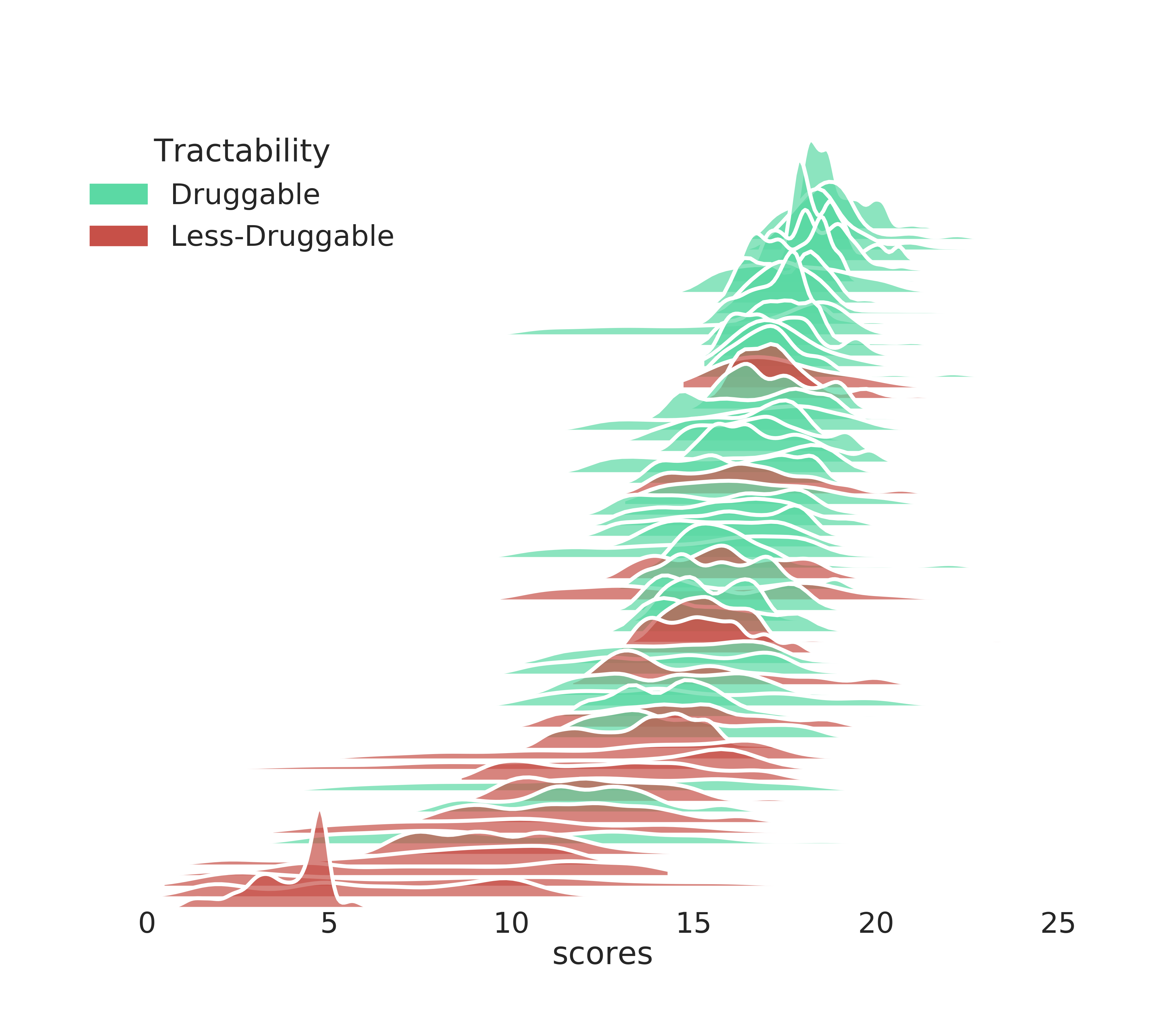
We can visualise the score distributions using the seaborn plotting library and use the ccdc.descriptors module for statical analysis on the ranked pockets.
JoyPlot
# adapted from the seaborn documentation.
#
import matplotlib.patches as patches
import matplotlib.pyplot as plt
import seaborn as sns

def joyplot(df, fname='test.png'):
    """
    Visualises the Fragment Hotspot Maps score distributions as
    a series of stacked kernal density estimates ordered by
    median value.

    Adapted from the seaborn gallery:
        https://seaborn.pydata.org/examples/kde_ridgeplot.html

    :param `pandas.DataFrame` df: Fragment Hotspot scores data
    :return None
    """
    sns.set(style="white",
            rc={"axes.facecolor": (0, 0, 0, 0)},
            font_scale=6)

    palette = ["#c75048",
               "#5bd9a4"
               ]

    # Initialize the FacetGrid object
    ax = sns.FacetGrid(df,
                       row="pdb",
                       hue="tractability",
                       height=4,
                       aspect=75,
                       palette=palette)

    # Draw the densities in a few steps
    ax.map(sns.kdeplot, "scores", clip_on=False, shade=True, alpha=.7, lw=3, bw=.2)
    ax.map(sns.kdeplot, "scores", clip_on=False, color="w", lw=9, bw=.2)

    # Format the plots
    ax.set(xlim=(0, 25))  #
    ax.fig.subplots_adjust(hspace=-.9)
    ax.set_titles("")
    ax.set(yticks=[])
    ax.despine(bottom=True, left=True)

    # Create legend, and position
    tag = {"d": "Druggable", "n": "Less-Druggable"}
    labels = [tag[s] for s in set(df["tractability"])]
    handles = [patches.Patch(color=col, label=lab)
               for col, lab in zip(palette, labels)]

    legend = plt.legend(handles=handles,
                        title='Tractability',
                        loc="upper right",
                        bbox_to_anchor=(0.3, 7.5))
    frame = legend.get_frame()
    frame.set_facecolor('white')
    frame.set_edgecolor('white')

    plt.savefig(fname)
    plt.close()

df = pd.read_csv('scores.csv')
df = df.sort_values(by='median', ascending=False)
joyplot(df, 'druggable_joy.png')
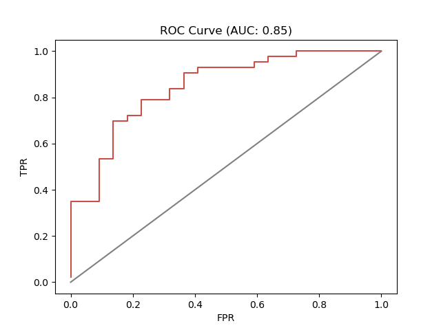
Rank Statistics
import operator
import seaborn as sns

from ccdc.descriptors import StatisticalDescriptors as sd


def rocplot(data, fname='roc.png'):
    """
    Create a ROC Curve using seaborn

    :param lists data: supply ranked data as list of list
    :return: None
    """
    rs = sd.RankStatistics(scores=data, activity_column=operator.itemgetter(2))
    tpr, fpr = rs.ROC()
    ax = sns.lineplot(x=fpr, y=tpr, estimator=None, color="#c75048")
    ax = sns.lineplot(x=[0,1], y=[0,1], color="grey")
    ax.set(xlabel='FPR', ylabel='TPR', title=f"ROC Curve (AUC: {rs.AUC():.2f})")

    plt.savefig(fname)
    plt.close()

df = pd.read_csv('scores.csv')

t = []
m = []
letter_to_number = {"d": 1, "n": 0}
for p in set(df['pdb']):
    a = df.loc[df['pdb'] == p]
    t.append(letter_to_number[list(a['tractability'])[0]])
    m.append(list(a['median'])[0])

df = pd.DataFrame({'tractability': t,  'median':m})
df = df.sort_values(by='median', ascending=False)
data = list(zip(list(df["median"]), list(df["tractability"])))

rocplot(data, fname='druggable_roc.png')
Hotspot-Guided Docking
Molecular docking is a staple of early-stage hit identification. When active small molecules are known, key interactions can be selected to steer the scoring of molecular pose to favour those molecules making the selected interaction. Fragment Hotspot maps can predict critical interactions in the absence of binding data. Using these predictions as constraints will likely improve docking enrichment. A preliminary study was conducted by (Radoux, 2018) and a full validation is currently underway. Protein Kinase B (AKT1) has been chosen for this tutorial example and was used in the prelimenary docking study.
Radoux, C. J. The Automatic Detection of Small Molecule Binding Hotspots on Proteins Applying Hotspots to Structure-Based Drug Design. (2018). doi:10.17863/CAM.22314
A Hotspot Constraint
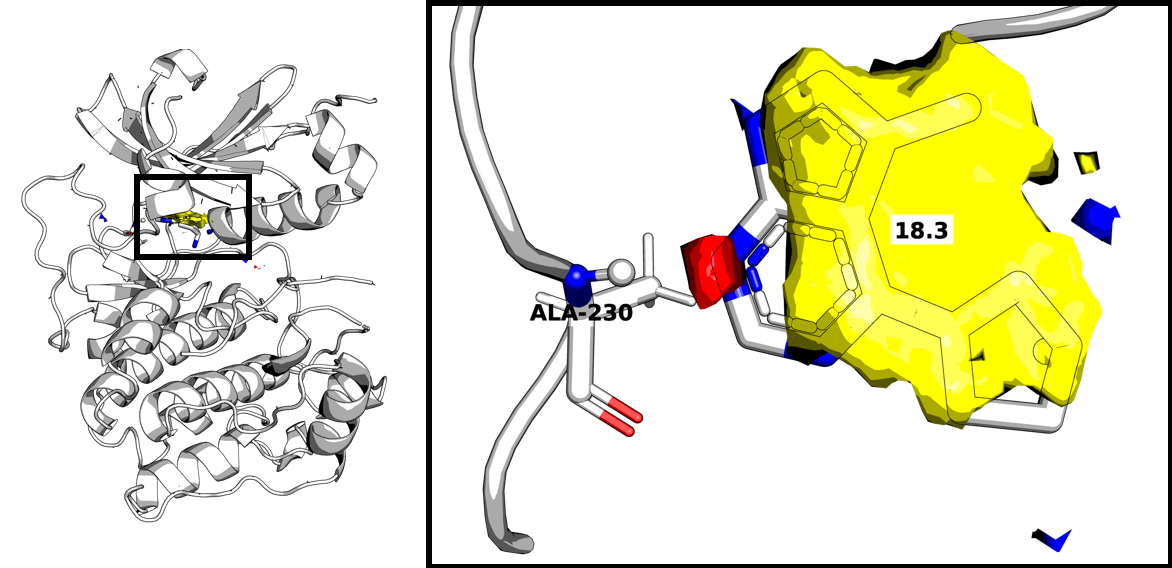
To begin, a hotspot calculation is performed on AKT1 (PDB: 3cqw). For this example, the protein was protonated using X, all waters, ligands and metal centres were removed.
hotspots.hsdocking.DockerSettings inherits from ccdc.docking.Docker.Settings to allow smooth integration with the CCDC python API. The following code snippet demonstrates how a constraint is generated and added to the hotspots.hsdocking.DockerSettings class.
from hotspots.hs_docking import DockerSettings
from hotspots.hs_io import HotspotReader


result = HotspotReader(<pathtohotspot>).read()

docker = Docker()
docker.settings = DockerSettings()
docker.settings.add_protein_file(<pathtoprotein>)

constraints =
docker.settings.HotspotHBondConstraint.create(protein=docker.settings.proteins[0],
                                                            hr=result,
                                                            weight=10,
                                                            min_hbond_score=0.05,
                                                            max_constraints=1)
for constraint in constraints:
    docker.settings.add_constraint(constraint)
View the Constraints
The automatic hotspot constraints are designed to be used unsupervised, as part of large scale docking studies where it is not practical to assess every protein manually. However, if you are studying a small number of proteins, you may want to view the suggested hydrogen bond constraints before running GOLD docking.
hotspot = "<path to hotspot out.zip>"
hotspot = HotspotReader(hotspot).read()

for p, g in hotspot.super_grids.items():
    hotspot.super_grids[p] = g.max_value_of_neighbours()

    # grayscale dilation used for noise reduction

constraints = hotspot._docking_constraint_atoms(max_constraints=5,
                                                max_distance=4,
                                                threshold=17,
                                                min_size=8
                                                )

# max_constraints: limits the number of constraints selected
# max_distance: island cenrtroid must be within max_distance to be selected
# threshold: hotspots contoured a threshold score
# min_size: island must have > min_size grid points to be selected

mol = constraints.to_molecule()

with MoleculeWriter("constraints.mol2") as w:
    w.write(mol)
The docking constraints generated from the hotspots can be converted into a ccdc.molecule.Molecule object and then easily visualised in a molecular visualing program. We use PyMOL. In this case, 1 hydrogen bond donor constraint is selected and therefore there is no selection to be made.
GOLD Docking
With the modified docking settings class, the rest of the docking calculation is carried out in a similar manner to any other GOLD API docking. A full run script is provided below, which has been adapted from the CCDC API documentation.
https://downloads.ccdc.cam.ac.uk/documentation/API/cookbook_examples/docking_examples.html
def dock(inputs):
    """
    submit a GOLD API docking calculation using
    docking constraints automatically generated
    from the Hotspot API

    :param ligand_path:
    :param out_path:
    :param hotspot:
    :param weight:
    :return:
    """
    def add_ligands(docker, ligand_path):

        with gzip.open(os.path.join(ligand_path,
                                    "actives_final.mol2.gz"), 'rb') as f_in:

            with open(os.path.join(docker.settings.output_directory,
                                    "actives_final.mol2"), 'wb') as f_out:
                shutil.copyfileobj(f_in, f_out)

        with gzip.open(os.path.join(ligand_path,
                                    "decoys_final.mol2.gz"), 'rb') as f_in:
            with open(os.path.join(docker.settings.output_directory,
                                   "decoys_final.mol2"), 'wb') as f_out:
                shutil.copyfileobj(f_in, f_out)

        docker.settings.add_ligand_file(os.path.join(docker.settings.output_directory,
                                                     "actives_final.mol2"),
                                        ndocks=5)

        docker.settings.add_ligand_file(os.path.join(docker.settings.output_directory,
                                                     "decoys_final.mol2"),
                                        ndocks=5)

    def add_protein(docker, hotspot, junk):

        pfile = os.path.join(junk, "protein.mol2")
        with MoleculeWriter(pfile) as w:
            w.write(hotspot.protein)

        docker.settings.add_protein_file(pfile)

    def define_binding_site(docker, ligand_path):

        crystal_ligand = MoleculeReader(os.path.join(ligand_path,
                                                     "crystal_ligand.mol2")
                                         )[0]
        docker.settings.binding_site =
        docker.settings.BindingSiteFromLigand(protein=docker.settings.proteins[0],
                                              ligand=crystal_ligand)

    def add_hotspot_constraint(docker, hotspot, weight):

        if int(weight) != 0:
            constraints =
            docker.settings.HotspotHBondConstraint.create(protein=docker.settings.proteins[0],
                                                          hr=hotspot,
                                                          weight=int(weight),
                                                          min_hbond_score=0.05,
                                                          max_constraints=1)

            for constraint in constraints:
                docker.settings.add_constraint(constraint)

    def write(docker, out_path):

        results = Docker.Results(docker.settings)

        # write ligands
        with MoleculeWriter(os.path.join(out_path, "docked_ligand.mol2")) as w:
            for d in results.ligands:
                w.write(d.molecule)

        # copy ranking file
        #
        # in this example, this is the only file we use for analysis.
        # However, other output files can be useful.

        copyfile(os.path.join(junk, "bestranking.lst"),
                 os.path.join(out_path, "bestranking.lst"))

    # GOLD docking routine
    ligand_path, out_path, hotspot, weight, search_efficiency = inputs
    docker = Docker()

    # GOLD settings
    docker.settings = DockerSettings()
    docker.settings.fitness_function = 'plp'
    docker.settings.autoscale = search_efficiency
    junk= os.path.join(out_path, "all")
    docker.settings.output_directory = junk

    # GOLD write lots of files we don't need in this example
    if not os.path.exists(junk):
        os.mkdir(junk)
    docker.settings.output_file = os.path.join(junk, "docked_ligands.mol2")

    # read the hotspot
    hotspot = HotspotReader(hotspot).read()
    for p, g in hotspot.super_grids.items():
        hotspot.super_grids[p] = g.max_value_of_neighbours()
        # dilation to reduce noise

    add_ligands(docker,ligand_path)
    add_protein(docker, hotspot, junk)
    define_binding_site(docker, ligand_path)
    add_hotspot_constraint(docker, hotspot, weight)

    docker.dock(file_name=os.path.join(out_path, "hs_gold.conf"))
    write(docker, out_path)

    # Clean out unwanted files
    shutil.rmtree(junk)


def create_dir(path):
    if not os.path.exists(path):
        os.mkdir(path)
    return path


def main():

    ligand_path = '<path to input directory>'
    output_path =  '<path to output directory>'
    hotspot_path = '<path to out.zip>'
    constraint_weight = 10
    search_efficiency = 100

    dock(inputs=(ligand_path,
                 output_path,
                 hotspot_path,
                 constraint_weight,
                 search_efficiency))
Performance Demonstration
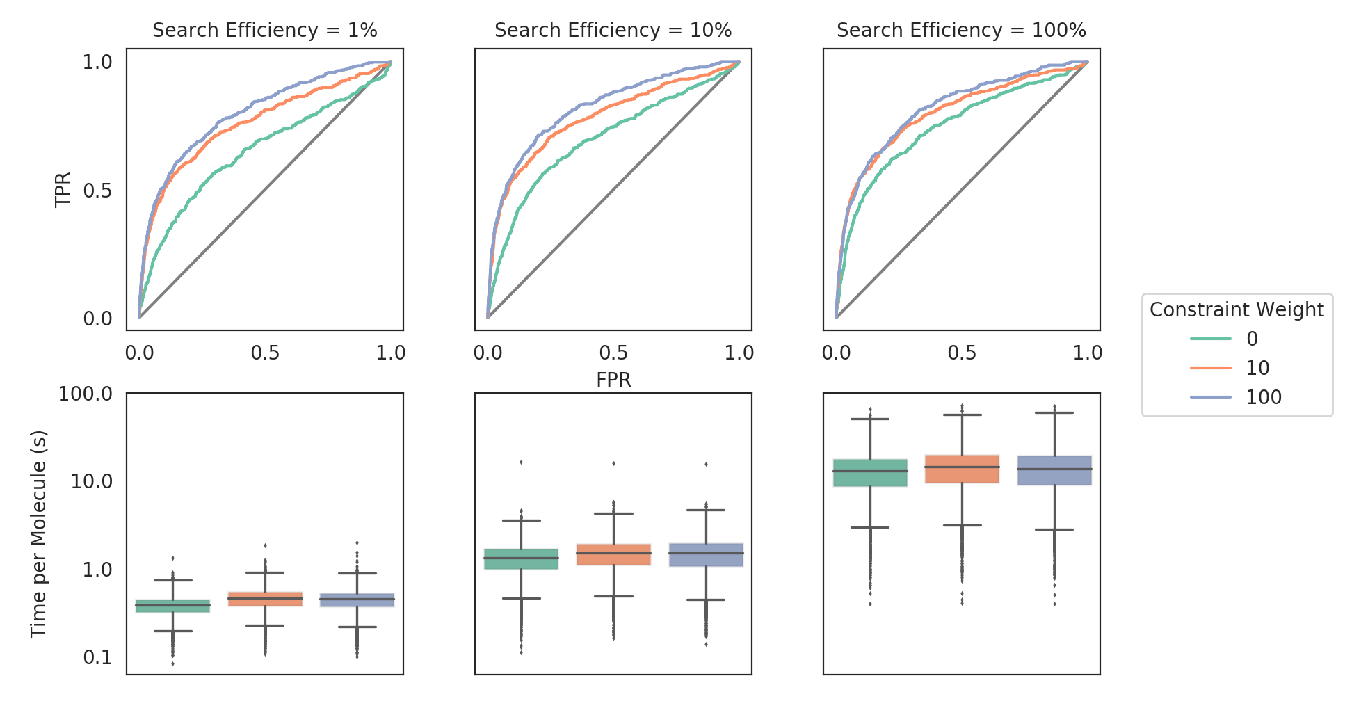
Using the code above, the AKT1 DUD-e set was docked against AKT1 (PDB: 3cqw), using the hotspot selected constraint (the amide hydrogen of ALA230). The docking calculations were run varying the weight of the protein hydrogen bond constraint [0, 10, 100] and the search efficiency [1, 10, 100].
The most significant effect is on retrieval speed. GOLD can be run using different search efficiencies which control the degree of sampling in the genetic algorithm. By using automated constraints, one can outperform 100% search efficiency results in 1% search efficiency settings; a speed improvement of more than an order of magnitude. While this work showcases this use case, we will undertake further work in future to evaluate the benefit more generally across a wider range of targets.
The code to generate the figure and statistics is given below.
import os

import numpy as np
import operator
import pandas as pd
import seaborn as sns
import matplotlib.pyplot as plt
from ccdc.descriptors import StatisticalDescriptors as sd

def rank_stats(parent, s, w):
    """
    Create two `pandas.DataFrame` from the "bestranking.lst"
    GOLD output

    :param str parent: path to parent directory
    :param str s: name of subdirectory
    :param str w: name of subsubdirectory
    :return:
    """
    # read data and process data from output file
    fname = os.path.join(parent,
                         f"search_efficiency_{s}",
                         str(w),
                         "bestranking.lst")
    lines = [l.strip("\n") for l in open(fname, "r").readlines()]
    header = lines[5]
    header = [b.strip() for b in
              [a for a in header.split("  ") if a != '' and a != '#']]
    all = lines[7:]

    cat = list(zip(*[[a for a in entry.split(" ") if a != '']
                     for entry in all]))

    # generate a dataframe and alter datatypes
    df = pd.DataFrame({h: cat[i] for i, h in enumerate(header)})
    df["actives"] = np.array(
        list(map(lambda x: 'CHEMBL' in x, list(df['Ligand name'])))
    ).astype(int)
    df["search_efficiency"] = [int(s)] * len(df)
    df["weight_int"] = [int(w)] * len(df)
    df["weight_str"] = [str(w)] * len(df)
    df["Score"] = df["Score"].astype(float)
    df["time"] = df["time"].astype(float)
    df["log_time"] = np.log10(list(df["time"]))
    df = df[['Score',
             'log_time',
             'actives',
             'search_efficiency',
             'weight_int',
             'weight_str']]
    df = df.sort_values(by=['Score'], ascending=False)

    # Use CCDC's descriptors API
    rs = sd.RankStatistics(scores=list(zip(list(df['Score']),
                                           list(df['actives']))),
                           activity_column=operator.itemgetter(1))

    # ROC
    tpr, fpr = rs.ROC()
    df["tpr"] = tpr
    df["fpr"] = fpr

    # Enrichment Metrics
    metric_df = pd.DataFrame({"search efficiency": [s],
                             "weight": [w],
                             "AUC": [rs.AUC()],
                             "EF1": [rs.EF(fraction=0.01)],
                             "EF5": [rs.EF(fraction=0.05)],
                             "EF10": [rs.EF(fraction=0.1)],
                             "BEDROC16": [rs.BEDROC(alpha=16.1)],
                             "BEDROC8": [rs.BEDROC(alpha=8)]
                             })
    return df, metric_df


def roc_plot(df, search_efficiency, ax, palette='Set2'):
    """
    Plot a ROC plot for the docking data

    :param `pands.DataFrame` df: data
    :param int search_efficiency: data is split by search efficiency
    :param `matplotlib.axes.Axes` ax: Matplotlib axis to plot data onto
    :param list palette: list of RGB tuples
    :return:
    """

    selected = df.loc[df['search_efficiency'] == search_efficiency]
    # random
    sns.lineplot(x=[0, 1], y=[0, 1], color="grey", ax=ax)
    # docking rank

    d = {"0": {"color": sns.color_palette(palette)[0],"linestyle": "-"},
         "10": {"color": sns.color_palette(palette)[1],  "linestyle": "-"},
         "100": {"color": sns.color_palette(palette)[2], "linestyle": "-"}}

    lines = [ax.plot(grp.fpr, grp.tpr, label=n, **d[n])[0]
             for n, grp in selected.groupby("weight_str")]


    ax.set_ylabel("")
    ax.set_xlabel("")
    ax.set_xticks([0, 0.5, 1])
    ax.set_title(label=f"Search Efficiency = {search_efficiency}%",
                 fontdict={'fontsize':10})

    return lines


def box_plot(df, search_efficiency, ax, palette='Set2'):
    """
    Plot a boxplot for the docking time data

    :param `pands.DataFrame` df: data
    :param int search_efficiency: data is split by search efficiency
    :param `matplotlib.axes.Axes` ax: Matplotlib axis to plot data onto
    :param list palette: list of RGB tuples
    :return:
    """

    selected = df.loc[df['search_efficiency'] == search_efficiency]
    sns.boxplot(x="weight_int", y="log_time", order=[0,10,100],data=selected,
                palette=palette,linewidth=1.2, fliersize=0.5, ax=ax)
    ax.set_ylabel("")
    ax.set_xlabel("")
    ax.set_xticks([])

    # just for asthetics
    for patch in ax.artists:
        r,g,b,a = patch.get_edgecolor()
        patch.set_edgecolor((r,g,b,.1))


def _asthetics(fig, axs, lines):
    """
    Extra formatting tasks

    :param `matplotlib.figure.Figure` fig: mpl figure
    :param list axs: list of  `matplotlib.axes.Axes`
    :param `matplotlib.lines.Line2D` lines: ROC lines
    :return:
    """
    # format axes
    axs[0][0].set_yticks([0, 0.5, 1])
    yticks = [-1, 0, 1, 2]
    axs[1][0].set_yticks(yticks)
    axs[1][0].set_yticklabels([str(10 ** float(l)) for l in yticks])
    axs[0][1].set_xlabel("FPR")
    axs[0][0].set_ylabel("TPR")
    axs[1][0].set_ylabel("Time per Molecule (s)")
    # format legend
    fig.legend(lines,
               [f"{w}" for w in [0,10,100]],
               (.83, .42),
               title="Constraint Weight")
    # format canvas
    plt.subplots_adjust(left=0.1, right=0.8, top=0.86)

def main():
    # read and format the data
    search_effiencies = [1, 10, 100]
    weights = [0, 10, 100]
    parent = "/vagrant/github_pkgs/hotspots/examples/" \
             "2_docking/virtual_screening/akt1/"

    df1, df2 = zip(*[rank_stats(parent, s, w)
                     for s in search_effiencies for w in weights])

    # Plotted Data (ROC and Box plots)
    df1 = pd.concat(df1, ignore_index=True)

    # Table Data (Rank Stats: AUC, EF, BEDROC)
    df2 = pd.concat(df2, ignore_index=True)
    df2.to_csv('rankstats.csv')

    # Plot the ROC and box plots
    sns.set_style('white')
    fig, axs = plt.subplots(nrows=2,
                            ncols=3,
                            sharey='row',
                            gridspec_kw={'wspace':0.26,
                                         'hspace':0.22},
                            figsize=(10,6), dpi=200)

    for i, row in enumerate(axs):
        for j, ax in enumerate(row):
            if i == 0:
                lines = roc_plot(df1, search_effiencies[j], ax)
            else:
                box_plot(df1, search_effiencies[j], ax)

    _asthetics(fig, axs, lines)
    plt.savefig("new_grid.png")
    plt.close()

if __name__ == "__main__":
    main()
Pharmacophores
A Pharmacophore Model can be generated directly from a hotspots.result.Result :
from hotspots.calculation import Runner
r = Runner()
result = r.from_pdb("1hcl")
result.get_pharmacophore_model(identifier="MyFirstPharmacophore")
The Pharmacophore Model can be used in Pharmit or CrossMiner
result.pharmacophore.write("example.cm")   # CrossMiner
result.pharmacophore.write("example.json")    # Pharmit
The CSD Python API’s documentation details how the output a “.cm” file can be used for Pharmacophore searching in CrossMiner. See the link below for details.
https://downloads.ccdc.cam.ac.uk/documentation/API/descriptive_docs/pharmacophore.html